Background
Batch gradient descent is one of the types of optimization algorithms from the gradient descent family. It is widely used in machine learning and deep learning algorithms for optimizing a model for better prediction. To understand this algorithm, you should have some understanding of differential equations to find a gradient of the cost function.
Definition
The batch gradient descent algorithm calculates a gradient of the cost function for all the independent parameters (input data) passed to a model. Now, computed gradient value along with the learning rate passed to a model will be used to update the existing weights of the model. This way weights will be updated until the error in prediction is reduced to a minimum so that prediction will happen with a minimum error. The gradient is the value that tells us how much cost function changes when any feature weight is changed. It is also called a partial derivative in mathematical terms.
In Brief
In simple terms, while reducing an error through cost function, batch gradient descent helps us to teach our model a direction where an error reduces. By using that direction, our model will be able to find weights that will be used in more accurate predictions.
Because it calculates a gradient for a batch of all values at once, it is called a batch gradient descent.
Let’s go ahead and understand how the batch gradient descent works.
Diagram
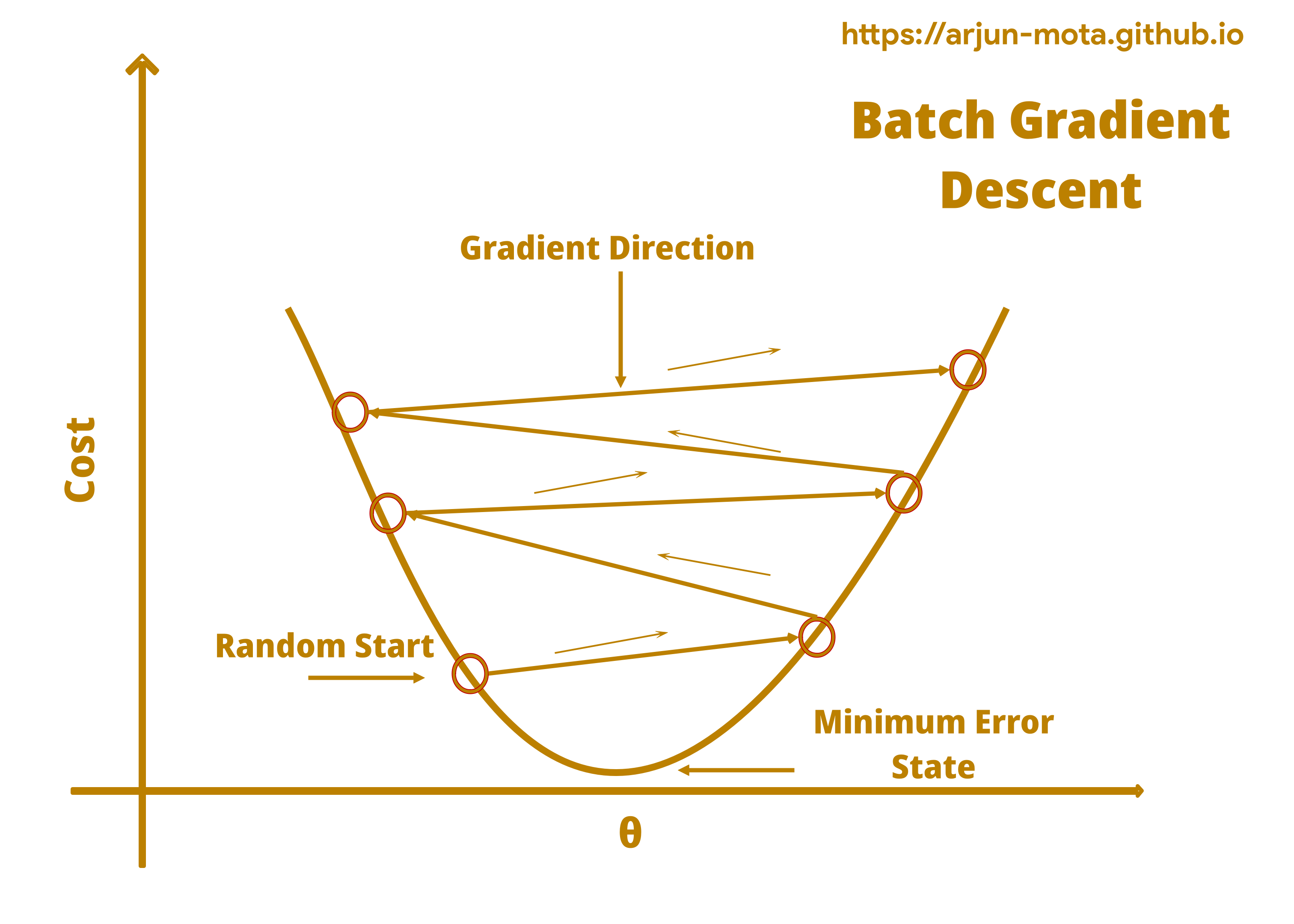
Batch Gradient Descent Direction Diagram

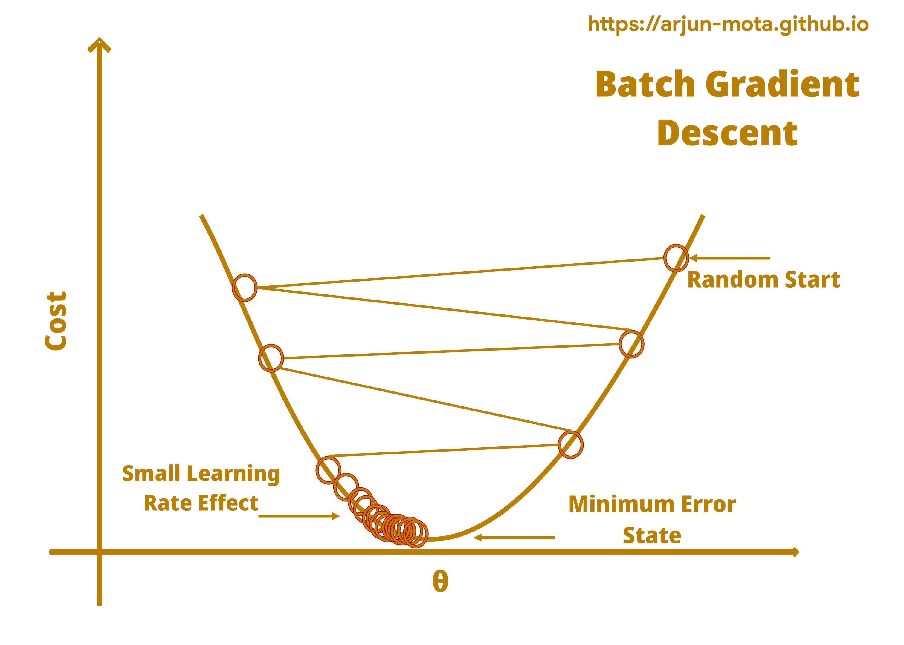
Batch Gradient Descent Convergence Diagram

Diagram > Explanation
• As we can see, weight changes the overall error in a prediction.
• We start with random weights and then optimize it to reduce an error through a batch gradient descent .
• In the diagram above, our algorithm moves from the left and right side of a curve while dealing with different weights.
• Using learning rate model parameter new weights will get assigned to features and the model reacts to those weights in terms of change in an error.
• Our goal is to find weights with minimum error, as the new weights are calculated our model goes down to reach the bottom which is the place for minimum error. Going downward is an ideal situation but it is not always true if the learning rate and our input data is not properly cleaned and scaled respectively.
• Learning rate is a very important parameter to reach a bottom efficiently. You will understand more once we will discuss the learning rate further.
Just keep this pseudocode in mind for further explanation.
Pseudocode > Batch Gradient Descent
1
2
3
4
5
6
7
Steps:
    1. Initialize random feature weights.
    2. Calculate the gradient for all records.
    3. Adjust feature weights by calculating new weights.
    4. Use new weights for prediction and calculate an error.
    5. Repeat steps 2, 3, and 4 for adjusting feature weights and
       do it until an error no longer reduces or reached some iterations limit.
Math Behind
To find a gradient, we need to calculate a partial derivative of a cost function. Below is the formula for a partial derivative of a cost function for a single feature:
Partial Derivative of a Single Feature > Formula
$$ \frac{\partial}{\partial \theta_{j}} \operatorname{MSE}(\boldsymbol{\theta})=\frac{2}{n} \sum_{i=1}^{n}\left(\boldsymbol{\theta}^{T} \mathbf{x}^{(i)}-y^{(i)}\right) x_{j}^{(i)} $$
where, \( \frac{\partial}{\partial \theta_{j}} \operatorname{MSE}(\boldsymbol{\theta}) \) = partial derivative of a cost function with regards to the parameter \( \theta_{j} \). \( \theta_{j} \) is a weight of a feature.
\( \boldsymbol{n} \) = number of records or input data’s length
\( \boldsymbol{\theta}^{T} \) = transpose of a weight theta
\( \mathbf{x}^{(i)} \) = feature value from an input vector
\( y^{(i)} \) = actual value of dependent variable from an input vector
\( x_{j}^{(i)} \) = feature value from an input vector (for single feature it is same as \( x^{(i)} \) or we can say it is jth feature value from ith input vector)
The above formula is just to remember to know how a partial derivative is calculated, but we want to calculate a partial derivative for more than one feature. Hence following formula is used to compute a partial derivative of all in one go.
Partial Derivative of a Multiple Features > Formula
$$ \nabla_{\boldsymbol{\theta}} \operatorname{MSE}(\boldsymbol{\theta})=\left(\begin{array}{c} \frac{\partial}{\partial \theta_{0}} \operatorname{MSE}(\boldsymbol{\theta}) \cr \frac{\partial}{\partial \theta_{1}} \operatorname{MSE}(\boldsymbol{\theta}) \cr \vdots \cr \frac{\partial}{\partial \theta_{n}} \operatorname{MSE}(\boldsymbol{\theta}) \end{array}\right) $$ is then become the following short formula:
$$ \nabla_{\boldsymbol{\theta}} \operatorname{MSE}(\boldsymbol{\theta})=\frac{2}{n} \mathbf{X}^{T}(\mathbf{X} \boldsymbol{\theta}-\mathbf{y}) $$
I assume that you already understood the first formula from above two formulas, so just want to add to the first one that \( \theta_{0}\ to \ \theta_{n} \) indicates weights of multiple features from 0 to n. But as you can see we have new formula for computing all. Where,
\( \nabla_{\boldsymbol{\theta}} \operatorname{MSE}(\boldsymbol{\theta}) \) = (nabla) inverted triangle symbol indicates a gradient vector of partial derivatives of the cost function
n = number of records or input data’s length
\( \mathbf{X} \) = input data matrix
\( \mathbf{X}^{T} \) = transpose matrix of an input
\( \theta \) = weights of all the features
y = actual values of a dependent variable from an input
Explanation > Batch Gradient Descent
Partial Derivative of a Single Feature
• In the first formula, we are taking a transpose of a theta weight that is in one feature doesn’t change and multiplying it with input feature x to get a prediction.
• Then subtracting a prediction with actual value to get an error.
• Multiplying this error with the input value of a feature mentioned as \( x_{j}^{(i)} \).
• We will do this for all input records and take a sum of it.
• That sum will be multiplied with a result of \( \frac{2}{n} \) where n is the number of records.
• This entire calculation will give us a partial derivative of a cost function for a single feature.
• But in real-life situations, we rarely have to deal with a single feature, hence the formula mentioned after that is for multivariable partial deviation.
Remember that this formula is not a batch gradient descent. The gradient vector that we got from the calculations so far will be used in updating existing feature weights that we will see in a moment, but before that let’s understand how we can calculate a partial derivative of a cost function for multiple features.
Partial Derivative of a Multiple Features
• There are two formulas mentioned, but we have to deal with the second one only as the first formula is just an explanation for multiple partial derivative calculations derived from a single feature formula.
• Now, coming to the second formula where we are taking a transpose of an input x and multiplying with \( \frac{2}{n} \).
• Inside the braces, we are multiplying all the input values x with their weights \( \theta \) and subtracting it by actual values in y (dependent variable).
• After that multiplying both the values, we will get a partial derivative of a cost function for all records.
Alright, now we will see how the weights are updated after finding a partial derivative.
New Feature Weights > Updating Weights
• Till this point, we have our gradient vector in \( \nabla_{\boldsymbol{\theta}} \operatorname{MSE}(\boldsymbol{\theta}) \), and feature weights in \( \theta \).
• There is also one model parameter called a learning rate (lr), it is a floating-point value used for weight updates.
• So, now we will use the following formula to get new weights for our model:
$$ \boldsymbol{\theta}^{(\text {new weights})}=\boldsymbol{\theta}^{(\text {old weights})}-lr * \nabla_{\boldsymbol{\theta}} \operatorname{MSE}(\boldsymbol{\theta}) $$
• We will multiply gradient vector with learning rate and subtract it from old weights to get new weights.
• Once the new weights are calculated, again the entire process will be repeated until the model finds optimum values for the weights that give a minimum error in a prediction.
• Larger learning rate will make this algorithm take more time to reach the bottom as it may skip the minimum value at the bottom and move to another side.
• The learning rate decides the magnitude of a change in weights, if it is large then weights will be updated by a large margin and vice versa. So it has to be chosen properly by experimentation and evaluation.
That’s it for the batch gradient descent, we are at the end of this optimization algorithm.
Diagram > Batch Gradient Descent Minima Diagram

Diagram > Explanation
• With comparison to the first diagram, we can see a local and a global minima here.
• Direction of a model to reach a minimum error state is also not straightaway downhill instead there are different ups and downs present in this scenario.
• Local minima is a state in a gradient descent where a model considers that it reached the minimum error and stop going further.
• Global minima is an actual state where error goes to a minimum and ideally, a model should identify that.
• However, by using a batch gradient descent we are calculating gradient for all records at once and if the cost function is irregular then we will have one or more local minima and one global minima.
• In that case, a batch gradient descent will take a long time to reach the global minima or may never reach if the learning rate is not suited and an input data is not scaled properly.
Conclusion
As mentioned above, the problem with a batch gradient descent is that it will take a long time when a cost function is irregular. To overcome this issue, a stochastic gradient descent is introduced that calculates a gradient for a specific amount of records at each time.
The stochastic gradient descent is better at finding a global minima than a batch gradient descent.
Overall a batch gradient descent is an optimization algorithm that changed the way machine learning works and helped achieving greater results.
In modern machine learning frameworks, there are different variants of gradient descents based on new researches.
Though, it is very unlikely that you have to implement this algorithm from scratch as frameworks used in a model development have already implemented it.
So, you just have to pass some parameters and wait for it to do the magic!
End Quote
“A breakthrough in machine learning would be worth ten Microsofts.” - Bill Gates