
Background
Brief
Linear regression is an algorithm where machine learning actually starts. It is a very basic supervised learning algorithm used to predict a numerical value by finding optimum coefficients for a straight line, plane or hyperplane with a given independent variable(s). Here we will dive deep into single and multidimentional linear regression. Stay with me till the end.
Use Cases
Here independent variables consist of all the features that are required to predict a dependent variable. Let me give you some linear regression use cases for better understanding.
Examples
• Predicting the temperature of a day
• Predicting the number of products to be sold
• Predicting the expenses
• Predicting a growth rate
• Predicting the price of a house
Intuition
Example > House Price Prediction
Consider predicting house price, where house price is the dependent variable that we want to predict based on some independent variables contributing to it. Independent variables could be the number of bedrooms, location, is furnished or not, number of years old, etc.
Math Behind
Remember that linear regression works only with numerical values, so if your variables are categorical and useful for your model then encode them to numbers. There are certain ways of doing that, those will be covered in a different article. Let’s understand the intuition behind this algorithm. So, here is an equation behind it:
$$ y = mx + b $$
y = dependent variable that we want to predict (house price),
m = slope, weight or coefficient,
x = our input feature (e.g. number of bedrooms) remain constant (model parameter),
b = bias term/intercept (model parameter).
Cost Function > Single Linear Regression
Here the question is how m (coefficient) is calculated?
It is called least squares method, let’s see how it works: \begin{array}{cccc} \mathrm{m}=\frac{\sum[(x i-\bar{x})(y i-\bar{y})]}{\sum\left[(x i-\bar{x})^{2}\right]} \end{array}
here \( \bar{x} \) is mean of x and \(\bar{y}\) is mean of y. Sum of multiplied differences of x from it’s mean and y from it’s mean are divided by sum of squared differences of x from it’s mean.
If bias b is not given then it is calculated as below: \begin{array}{cccc} \mathrm{b}=\bar{y}-m * \bar{x} \end{array}
That’s it for linear regression with one feature, now when we will give a new data i.e. number of bedrooms as an input to our model, it will calculate y = mx + b and give us our output y which is called yhat. When we check an accuracy of our model we check the difference between output yhat and actual value y in our test data.
With y = mx + b equation, we can get a predicted value of y only if we have one independent variable/feature like the number of bedrooms in house price prediction.
In case of multiple features, we have to use multiple linear regression, have a look at the below equation for that: \begin{array}{cccc} y=b_{1} x_{1}+b_{2} x_{2} \ldots . . b_{n} x_{k}+b_{0} \end{array} In this case, calculation requires matrices as follows: $$ y = \pmatrix{ y_{1} \cr y_{2} \cr y_{3} \cr \vdots \cr y_{n} \cr } $$
$$ b = \pmatrix{ b_{0} \cr b_{1} \cr b_{2} \cr \vdots \cr b_{n} \cr } $$
$$ x = \pmatrix{ 1 & x_{11} & x_{12} & \ldots & x_{1k} \cr 1 & x_{21} & x_{22} & \ldots & x_{2k} \cr \vdots & \vdots & \vdots & \ldots & \vdots \cr \vdots & \vdots & \vdots & \ldots & \vdots \cr 1 & x_{n1} & x_{n2} & \ldots & x_{nk} \cr } $$
Unlike the first equation, here $$ y = x * b $$ because b contains \( b_{0} \) as bias term with all coefficients and given y is a matrix of all predicted values that we will have after doing this computations. x has 1’s in first column that will be scores of each record of our dataset, and rest are all the records. We have n records and k features/variables in this matrix.
Cost Function > Multi Linear Regression
So, how coefficients are calculated in multiple linear regression?
Below mentioned equation of computing coefficients of multiple linear regression is called least squares normal equation.
$$ b=\left(x^{T} x\right)^{-1} x^{T} y $$
here \( x^{T}\) is the transpose matrix of x, \( \left(x^{T} x\right)^{-1}\) is an inverse of \( \left(x^{T} x\right)\) matrix,
After putting all values in place, we will get coefficients in b, which are same as earlier discussed single feature bias term:
$$ \mathrm{b}=\bar{y}-m * \bar{x} $$
Alright, Well done! We are done with the math of multiple linear regression as well. Let’s look at following diagram showing how linear regression works visually.
Diagram
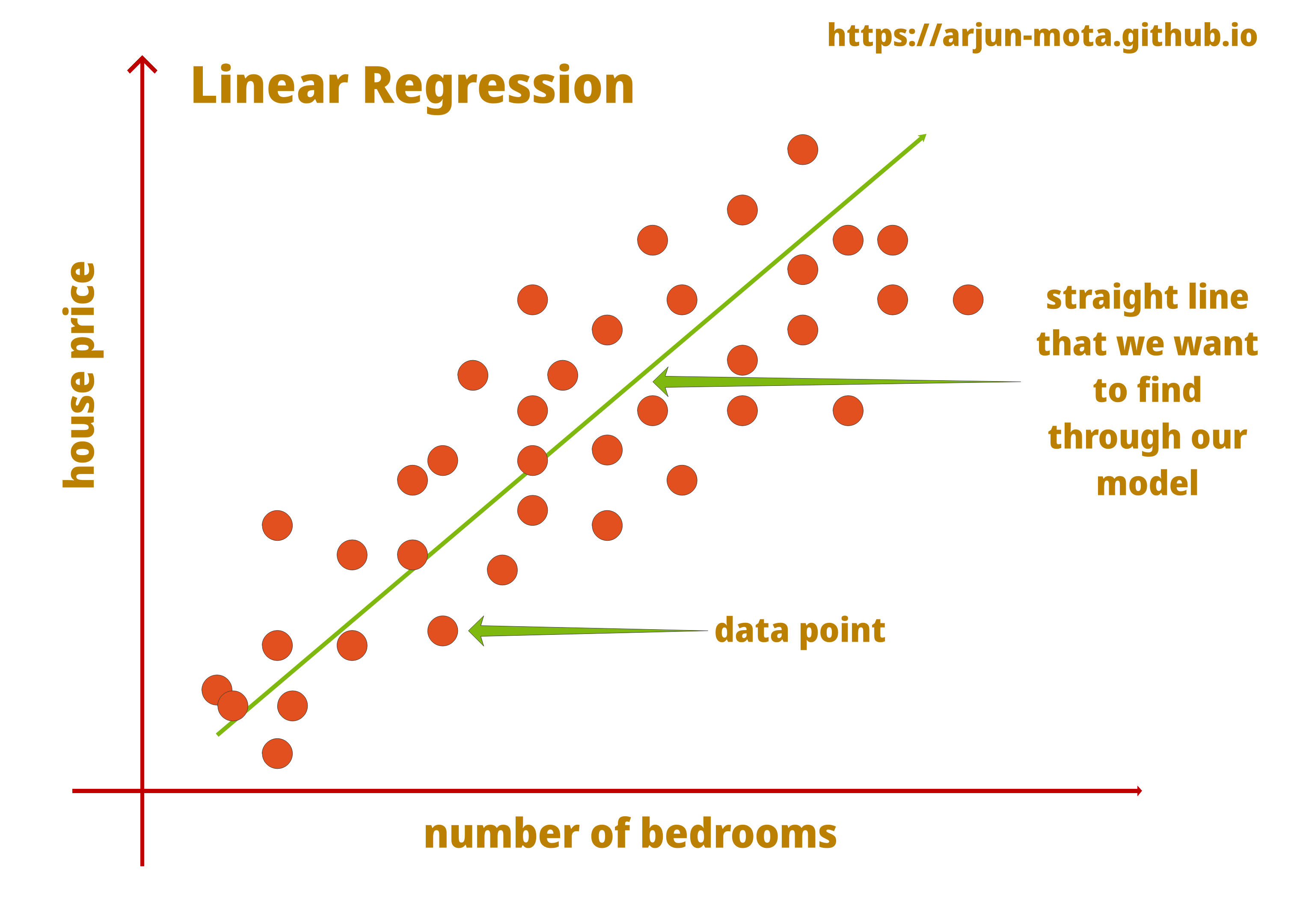
Details
We need to remember that it only works well when dependent and independent features are positively correlated and linearly separable. Here in the above graph, we can see the representation of linear regression data points on a straight line that shows how data distributed in different places, house price and number of bedrooms are also positively correlated as number of bedrooms increases house price also increases.
Conclusion
Our straight line of linear regression should cover most of the data points for better prediction. Better the straight line, less the error in prediction. But don’t misunderstand that we need to make sure it does not overfit, as it will result in an excellent performance on test data and very poor on new data. Our goal should be making a generalized model that works well with all kinds of data.
For evaluating our model, we can use various metrics like mean squared error [MSE], rooted mean squared error [RMSE], etc. I have covered different evaluation metrics in detail here: Evaluation Metrics. Keep checking my blog once in a while, new article will appear on a home page.
End Quote
“Machine intelligence is the last invention that humanity will ever need to make.” ~ Nick Bostrom