
Background
Brief
Logistic regression is one of the very first and popular algorithms for classification tasks. It is also a supervised machine learning algorithm meaning we need some actual outputs with input to learn from. Logistic regression is a probabilistic algorithm as it will give the final output based on the probability of a certain output from 0 to 1. Logistic regression uses a sigmoid function to do that.
Logistic regression has two major types: Binary Logistic Regression and Multinomial Logistic Regression. We will look at all these aspects of logistic regression in this article. Let us first understand some use cases of the logistic regression.
Use Cases
Logistic regression is mostly used in classification tasks where we need to classify between two output either Yes or No, True or False, 0 or 1, etc. Though, we can use multinomial logistic regression for more than two outputs.
Examples
• Predicting whether a certain team from a cricket match will win or lose
• Predicting whether tomorrow will rain or not
• Predicting whether a patient is positive or negative by infection
• Predicting whether a user will click on the link or not
• Predicting which player out of many will score the most goals in a football match
Intuition
Example > Prediting Whether a Certain Team From a Cricket Match Will Win or Lose
Let us consider that we want to predict that in a One Day International (ODI) cricket match between India and Australia at Wankhede Stadium, Mumbai whether India will win or lose. Several factors are affecting the result of a match like atmosphere on the match day, pitch condition, toss result, playing XI, past performance of players against Australia at the same stadium and elsewhere, the current performance of players, etc.
Let us understand how the logistic regression works in this kind of use case.
Math Behind
Logistic regression also takes a weighted sum of input features along with bias term just like Linear regression, but it will give us a probability. So to convert the weighted sum to probability it uses a sigmoid function which outputs a value between 0 to 1 indicating probability from 0 to 100%.
Let us first understand the below formula for finding probabilities for output types.
Probability Estimation
$$ \hat{p}=\sigma\left(b_{1} x_{1}+b_{2} x_{2} \ldots . . b_{n} x_{k}+b_{0}\right) $$
Here, \( \hat{p} = \) (p hat) probability of output types (true/false, yes/no, win/lose)
\( \sigma = \) sigmoid function
b = bias term and coefficients
x = input features
As discussed earlier, the weighted sum of input features along with bias term passed to the sigmoid function to get a probability.
Let us understand the sigmoid function now.
Probability Estimation > Sigmoid Function
$$ \sigma(t)=\frac{1}{1+\exp (-t)} $$
Here, \( \sigma(t) = \) sigmoid output of t input
t = weighted sum of input features with bias term as explained in earlier equation \( \left(b_{1} x_{1}+b_{2} x_{2} \ldots . . b_{n} x_{k}+b_{0}\right) \)
\( \exp = \) exponential function
This sigmoid function will give us an output between 0 and 1.
Probability Estimation > Output
After getting probabilities, output will be converted to 0 or 1 based on the following calculation:
$$ \hat{y}=\begin{cases} 0 \text { if } \hat{p} < 0.5 \ \cr 1 \text { if } \hat{p} \geq 0.5 \ \cr \end{cases} $$
if the probability is less than 0.5 than it is considered as 0 or false or lose, etc, and
if the probability is greater than or equal to 0.5 than it is considered as 1 or true or win etc;
This would be our final output from the logistic regression algorithm.
Now, let us understand how input feature weights are optimized using a cost function.
Cost Function > Partial Derivative of Single Feature
$$ \frac{\partial}{\partial \theta_{j}} \mathrm{J}(\boldsymbol{\theta})=\frac{1}{n} \sum_{i=1}^{n}\left(\sigma\left(\boldsymbol{\theta}^{T} \mathbf{x}^{(i)}\right)-y^{(i)}\right) x_{j}^{(i)} $$
\( \theta_{j} \) is a weight of a feature.
\( \sum \) symbol for doing summation.
\( \boldsymbol{n} \) = number of records or input data’s length
\( \sigma \) = sigmoid function
\( \boldsymbol{\theta}^{T} \) = transpose of a weight theta
\( \mathbf{x}^{(i)} \) = feature value from an input vector
\( y^{(i)} \) = actual value of dependent variable from an input vector
\( x_{j}^{(i)} \) = feature value from an input vector (for single feature it is same as \( x^{(i)} \) or we can say it is jth feature value from ith input vector)
The above cost function will give us a partial derivative of a single feature. After calculating for all features we can use them to update existing weights. There is not any formula for calculating all features partial derivatives in one go that I know.
Refer partial derivative calculations for single and multiple features in batch gradient descent here for better understanding: Batch Gradient Descent Partial Derivative Calculations
Once we have all the partial derivatives, we can use them in gradient descent algorithms to find optimum feature weights.
Refer Gradient Descent Algorithms
That’s all for logistic regression, you can now use it in solving your problems.
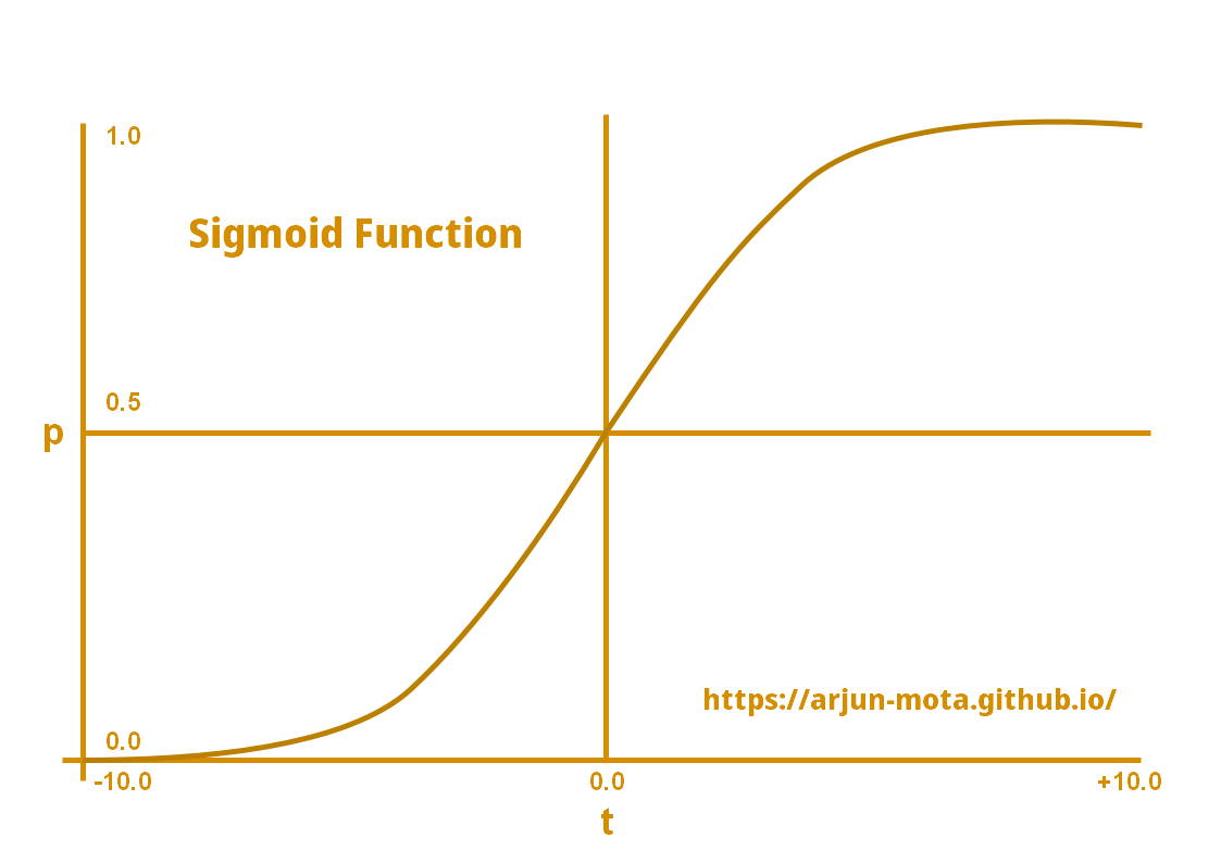
Following is an illustration of how sigmoid function outputs 0 or 1 from probabilities.
Diagram > Sigmoid Function
Details
• As you can see in the diagram, positive t values will have probability greater than or equal to 0.5 and they will become 1 in the final output.
• Whereas on the other side negative t values will have probabilities less than 0.5 that will become 0 in the final output.
• Sigmoid function gives us the “S” shaped curve.
Logistic Regression > Things To Remember
• Now, you know how to use logistic regression, but what about determining the accuracy of the model?
• An accuracy of a classification model can be measured with different evaluation metrics.
• Some of them are Confusion matrix, ROC curve, F1 Score, etc.
• Evaluation metrics are not covered in this article, but they will be available in detail in future articles and will be linked here.
• Now, talking about the implementation of logistic regression, the sklearn library of python has already implemented it so you just have to pass some parameters to use that.
• It has also an implementation of binary and multinomial logistic regression by changing a few parameters.
• Binary logistic regression is the one that we have discussed in this article but multinomial is the one where we have more than 2 output types.
• For multinomial logistic regression, softmax function is used that will give a probability for all the output types just like sigmoid function for two output types.
• Softmax function will be discussed in a future article and it will be linked here as well.
• We can also use polynomial features here in logistic regression for better performance. Check here Polynomial Regression for understanding how we can transform normal features to polynomial features.
Conclusion
• Logistic regression is easy to implement and does not require huge computation power.
• It is easy to interpret therefore used widely in corporate projects.
• It works well when the problem is linear and features are correlated to the output variable.
• If you want to use non-linear features, then you must transform them.
That is how the logistic regression works. Try using it with your use cases and see how it behaves.
End Quote
Machine learning is the science of getting computers to learn without being explicitly programmed. – Sebastian Thrun